Tutorial

import rayXpanda
import numpy as np

/=================\
|    rayXpanda    |
|-----------------|
|   Version: 0.1  |
\=================/

We call the functions like so:

u = 0.5
cos_alpha = 0.5

cos_psi = rayXpanda.deflection.deflect(cos_alpha, u)[0]

rayXpanda.inversion.invert(cos_psi, u)

(0.5000000000000001, 1.0175735797883876)

Let’s time the vectorised versions:

cos_alpha = np.linspace(-0.05, 1.0, 1000)

%%timeit -n100 -r100

rayXpanda.deflection.deflect_vec(cos_alpha, 0.5)

100 loops, best of 100: 128 µs per loop

cos_psi = np.linspace(-0.5, 1.0, 1000)

%%timeit -n100 -r100

rayXpanda.inversion.invert_vec(cos_psi, 0.5)

100 loops, best of 100: 707 µs per loop

We can examine the performance of invert():

from matplotlib import pyplot as plt
from matplotlib import rcParams
from matplotlib.ticker import MultipleLocator, LogLocator, NullFormatter
from matplotlib import gridspec

rcParams['text.usetex'] = False
rcParams['font.serif'] = 'Computer Modern Roman'
rcParams['font.family'] = 'serif'
rcParams['font.size'] = 16.0

fig = plt.figure(figsize=(12,12))

gs = gridspec.GridSpec(2, 2, height_ratios=[1,1], width_ratios=[1,1],
                       hspace=0.075, wspace=0.25)
ax_rays = plt.subplot(gs[0,0])
ax_error = plt.subplot(gs[1,0])

ax_deriv = plt.subplot(gs[0,1])
ax_deriv_e = plt.subplot(gs[1,1])

ax_rays.set_ylabel(r'$\cos\alpha$')
ax_error.set_xlabel(r'$1+\cos\psi$')
ax_error.set_ylabel(r'$|\varepsilon|$')

ax_deriv.set_ylabel(r'$\partial\cos\alpha/\partial\cos\psi/(1-u)$')
ax_deriv_e.set_xlabel(r'$1+\cos\psi$')

ax_rays.yaxis.set_major_locator(MultipleLocator(0.2))
ax_rays.yaxis.set_minor_locator(MultipleLocator(0.05))
ax_error.yaxis.set_major_locator(MultipleLocator(0.2))
ax_error.yaxis.set_minor_locator(MultipleLocator(0.05))

###

def add_u(u, color, lw=0.5):

    cos_psis = np.linspace(-0.999, 0.999, 1000)
    cos_alphas, deriv = rayXpanda.inversion.invert_vec(np.copy(cos_psis), u)
    cos_psis_defl, deriv_defl = rayXpanda.deflection.deflect_vec(np.copy(cos_alphas), u)

    ax_rays.plot(1.0+cos_psis, cos_alphas, color=color, ls='-', lw=lw, label=r'inversion: $u=%.3f$'%u)
    ax_deriv.plot(1.0+cos_psis, deriv, color=color, ls='-', lw=lw)

    ax_rays.plot(1.0+cos_psis_defl, cos_alphas, color=color, ls='-.', lw=lw, label=r'deflection: $u=%.3f$'%u)
    ax_deriv.plot(1.0+cos_psis_defl, deriv_defl, color=color, ls='-.', lw=lw)

    ax_error.plot(1.0+cos_psis, np.abs((np.arccos(cos_psis) - np.arccos(cos_psis_defl)))/np.arccos(cos_psis), color=color, ls='-', lw=lw)

    ax_deriv_e.plot(1.0+cos_psis, np.abs((deriv - deriv_defl))/deriv, color=color, ls='-', lw=lw)

###

add_u(5./8., 'r', 0.5)
add_u(0.5, 'k', 0.5)
add_u(0.4, 'b', 0.5)

###

ax_rays.set_xscale('log')
ax_rays.set_xticklabels([])
ax_rays.set_xlim([1.0e-2,2.0])
ax_rays.set_ylim([-0.4,1.0])

ax_error.set_yscale('log')
ax_error.set_xscale('log')
ax_error.set_ylim([1.0e-8,0.1])
ax_error.set_xlim([1.0e-2,2.0])

locmaj = LogLocator(base=100.0, numticks=100)
ax_error.yaxis.set_major_locator(locmaj)

locmin = LogLocator(base=100.0, subs=[0.02, 0.04, 0.06, 0.08, 0.1, 0.2, 0.4, 0.6, 0.8],
                    numticks=100)
ax_error.yaxis.set_minor_locator(locmin)
ax_error.yaxis.set_minor_formatter(NullFormatter())

ax_deriv.set_xscale('log')
ax_deriv.set_yscale('log')
ax_deriv.set_ylim([1.0,10.0])
ax_deriv.set_xlim([1.0e-2,2.0])
ax_deriv.set_xticklabels([])

ax_deriv_e.set_yscale('log')
ax_deriv_e.set_xscale('log')
ax_deriv_e.set_ylim([1.0e-8,1.0])
ax_deriv_e.set_xlim([1.0e-2,2.0])

locmaj = LogLocator(base=100.0, numticks=100)
ax_deriv_e.yaxis.set_major_locator(locmaj)

locmin = LogLocator(base=100.0, subs=[0.02, 0.04, 0.06, 0.08, 0.1, 0.2, 0.4, 0.6, 0.8],
                    numticks=100)
ax_deriv_e.yaxis.set_minor_locator(locmin)
ax_deriv_e.yaxis.set_minor_formatter(NullFormatter())
ax_deriv.yaxis.set_minor_formatter(NullFormatter())

for x in [ax_rays, ax_error, ax_deriv, ax_deriv_e]:
    x.tick_params(which='major', colors='black', length=8)
    x.tick_params(which='minor', colors='black', length=4)
    x.xaxis.set_tick_params(which='both', width=1)
    x.yaxis.set_tick_params(which='both', width=1)
    plt.setp(x.spines.values(), linewidth=1, color='black')
    [i.set_color("black") for i in x.get_xticklabels()]
    [i.set_color("black") for i in x.get_yticklabels()]

_ = ax_rays.legend(loc=2, frameon=False, fontsize=10.0)

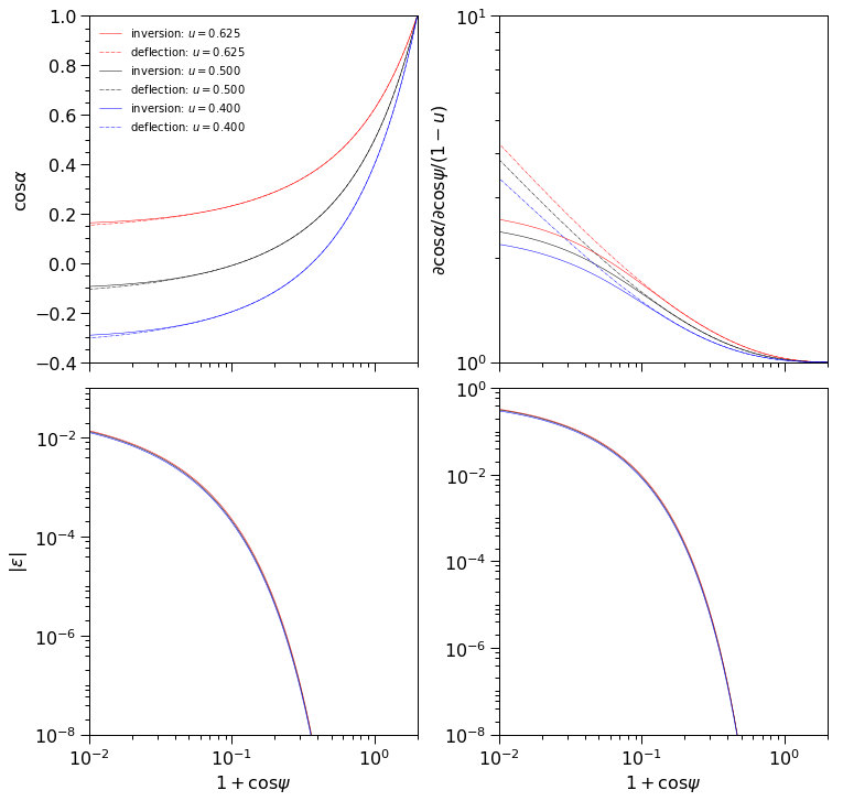
The fractional error is defined for the left panels as \(|\varepsilon|\mathrel{:=}|\psi-\tilde{\psi}|/\psi\). This choice is made because the map \(\cos\psi\mapsto\cos\alpha\) encoded by invert() is defined for primary images, returning for \(\cos\psi\in[-1,1]\) a positive value of the derivative

\[\mathcal{D}=\frac{1}{1-u}\frac{\partial\cos\alpha}{\partial\cos\psi},\]

with range \(\cos\alpha\in[a,1]\) where \(a\leq-1\).

However, the map encoded by deflect() has a domain \(\cos\alpha\in[b,1]\) for primary images where \(b\sim a\) is not known without additional calculation. Thus if \(\cos\alpha\notin[b,1]\) (i.e., \(\cos\alpha<b\)) then \(\cos\alpha\mapsto\cos\psi\) gives either \(\cos\psi\notin[-1,1]\), or \(\cos\psi\in[-1,1]\) and \(\mathcal{D}<0\).

Therefore, above we first called the (vectorised variant of) invert() with domain \(\cos\psi\in[-1,1]\) corresponding to \(\psi\in[-\pi,\pi]\). Then we called (the vectorised variant of) deflect() with domain \(\cos\alpha\in[a,1]\) to recover deflection angles \(\tilde{\psi}\). Note that the deflections \(\tilde{\psi}(\alpha)\) are more accurate with respect to the exact solutions (see the theory) than the angles \(\psi\).

Finito.